Reference manual¶

Architectural overview¶

Synopsis¶

The core functionality of the IDEAL software is to compute the dose distribution for any PBS ion beam treatment plan, using Geant4/GATE as the dose engine. The primary purpose is to provide an independent dose calculation tool that may be useful in clinics, but the software is designed to be useful also for a variety of research topics related to dose calculations.

Since Geant4/GATE simulations are quite CPU time consuming, IDEAL is designed to run on a GNU/Linux cluster in order to achieve the statistical goal within a reasonable time. IDEAL is implemented as a set of python modules and scripts. These convert the information in the input DICOM plan data into a set of data files and scripts that can be used by Gate to simulate the delivery of each of the beams requested in the treatment plan, using beamline model details and CT calibration curves that are configured by the user during installation and commissioning of the IDEAL. The dose distribution for each beam is computed separately up to the statistical goal specified by the user: number of primaries, average uncertainty or a fixed calculation time. The dose grid is by default the same as used by the treatment planning system, but the user can choose a different the spatial resolution by overriding the number of voxels per dimension. Each of the beam dose distributions as well as the plan dose distribution are exported as DICOM files.

In the following sections the key elements of this setup will be described in more details.

Device-oriented workflow¶

A device oriented example view of the workflow is illustrated in the figure below.

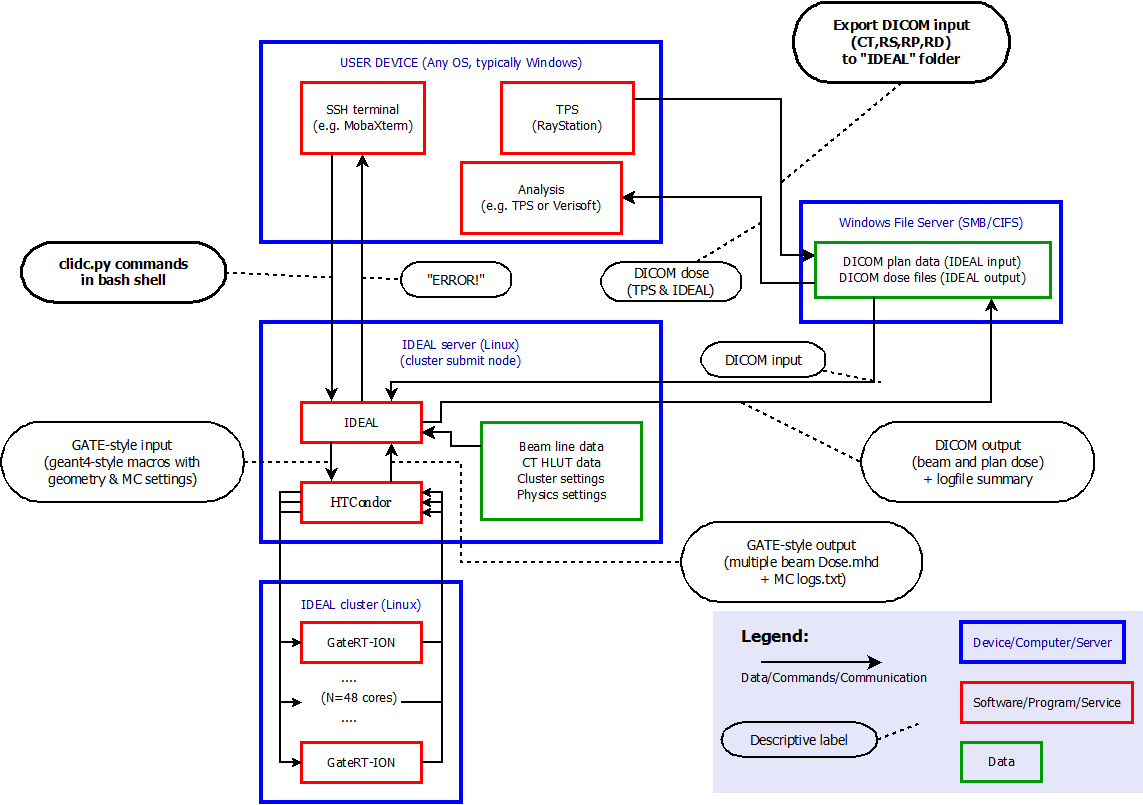
In this view, the user is logged in to the treatment planning workstation.

The user exports a treatment plan (or “beam set”) from the TPS to DICOM files on a shared file system. The exported data include the planning CT, the treatment plan (including the ion beam sequence), the structure set and physical and/or effective dose for the beams and/or the plan, in a folder that is also mounted on the submission node of the cluster.
The user logs in to the submission node of the cluster and runs one of the IDEAL user interface scripts (clidc.py or socrates.py) to start an independent dose calculation. The minimum input information is the treatment plan file and the statistical goal (number of primaries or average uncertainty). Optional overrides of the default settings are discussed in the following sections.
IDEAL collects and checks all necessary DICOM data that are referred to by the treatment plan file: the structure set (including exactly one ROI of type “External”), the planning CT and the TPS dose.
IDEAL finds the beamline model(s) corresponding to the treatment machine(s) specified in the plan file.
IDEAL finds the conversion tables for the CT protocol of the planning CT.
A ‘work directory’ is set up with all scripts specific for the IDC of the treatment plan: * configuration file for Preprocessing (CT image cropping, material overrides) * shell scripts, macros and input files for GateRTion * configuration file for Postprocessing (dose accumulation, resampling and export to DICOM) * submit file for HTCondor (cluster job management system) “DAGman” job.
The IDC is started by submitting the condor “DAGman” job. The directed acyclical graph (DAG) has just three nodes: * preprocessing on the submit node * Gate simulation on the calculation nodes * postprocessing on the submit node
A “job control daemon” is spawned which will regularly (default every 300 seconds) check whether the statistical goal (average uncertainty or number of primaries) has been reached for each successive beam. If the goal is reached, then a semaphore file “STOP-<beamname>” is created in the work directory. The scripts that are called by the Gate “StopOnScript” actor check the presence of that semaphore file to decide whether to stop the simulation or to continue.

Preprocessing¶

The job-dependent details for the preprocessing are computed and saved to a text file by ideal.impl.idc_details.WritePreProcessingConfigFile(). The preprocessing is performed by the bin/preprocess_ct_image.py script as part of the HTCondor DAGman corresponding to the IDC job.

Cropping: the minimum bounding box is computed that encloses both the “padded” External ROI volume in the planning CT and the TPS dose distribution. The External ROI is padded with a fixed thickness of air on all six sides. The padding thickness can be configured with an entry for air box margin [mm] in the [simulation] section of the system configuration file. This air-padding may help improving the correctness of skin dose calculation.
Hounsfield unit values are truncated to the maximum HU value specified in the density curve given for the relevant CT protocol.
In all voxels whose central point is not within the External ROI volume, the material is overridden with air (G4_AIR).
Each override specified by the IDEAL user is applied to all voxels whose central point lies within the ROI to which the override applies. The user should not specify different material overrides for two or more overlapping ROIs, since the order in which the overrides will be applied is random.
The material overrides are implemented by extending a copy of the interpolated Schneider table corresponding to the relevant CT protocol. In the extension, HU values larger than the maximum HU value in the density curve tables are associated with the override materials, and in the preprocessed CT image those high HU values are used for the voxels that have material overrides.
A mass file is created with the same geometry as the cropped CT image, with floating point voxel values representing the density (in grams per cubic centimeter). For voxels with material overrides (e.g. outside the external), the density value are taking from the overriding material; for all other voxels the density is obtained by a simple linear interpolation in the density curve.
A dose mask file is created with the same geometry as the output dose files, with value 1 (0) for all voxels with the central point inside (outside) the External ROI.

Gate simulation¶

Work directory: By convention, a Gate work directory has 3 subfolders named mac (Gate/Geant4 macro files with commands to define the specifics of the simulation), data (any input files that are usually not macro files) and output (all output goes into this folder). As we wish to run many instances of the same Gate job on a cluster, the corresponding output directories are suffixed with the job number. As IDEAL simulates each beam separately, there is a main macro file for each beam in the beam set. For a beam set with 3 beams, running on a cluster with 50 physical cores, 150 output directories are created.
Patient Geometry: The geometry for the simulation is defined in such a way that the isocenter coincides with the origin in the Geant4 coordinate system. A patientbox volume is defined as the smallest rectangular box that is centered on the isocenter and contains the (cropped) patient CT image plus a small air margin. The material of the world and patient box volumes is G4_AIR. This patient box helps to perform the translation and the rotation of the (cropped) CT image in the correct order: #. The (cropped CT) is imported into Gate using the ImageNestedParametrisedVolume geometry element defined by Geant4/Gate as a daughter volume of the patientbox. #. Using the TranslateTheImageAtThisIsoCenter configuration with the iso center coordinates taken from the DICOM plan data, the CT image is translated with respect to the origin of the patientbox. #. The couch rotation is performed on the patient box. The negative of the angle given in the DICOM plan file is used, to account for the difference in coordinate systems.
Phantom Geometry: For commissioning purposes, it can be useful to run the simulation on a geometrically defined phantom instead of the CT image that was specified in the DICOM plan file. To this end, the user specifies the name of a phantom that was configured during commissioning. The planned couch angle has no effect on the positioning of the phantom.

Hounsfield Units to materials conversion

IDEAL uses the recipe defined by [Schneider2000] to associate the Hounsfield Unit value of each CT voxel into a material with a suitable density and chemical composition. Geant4/Gate provides a HounsfieldMaterialGenerator to interpolate a density curve (specified as a sparse table of (HU,density) data points) and a ‘material composition file’ (list of mass fractions of chemical elements for about a dozen subsequent ranges of HU values) into

The CT protocol is deduced by applying the DICOM match criteria specified in the hlut.conf configuration file (as defined during commissioning) to (one of) the CT DICOM files. Each CT protocol is associated with a density curve and a Schneider style HU-to-composition table. Using the density tolerance value (given in system config file) and the HounsfieldMaterialGenerator in Geant4/Gate (…). If a CT protocol is used for the first time, or if the contents of the density and/or composition files have changed, and/or if the density tolerance value has changed, then set of interpolated materials and a table of HU values to these materials are generated and saved in the cached folder in the commissioning data directory, so that they can be reused

Nozzle and passive elements: For each treatment machine (beam line), the commissioning physicist should have provided Geant4/Gate macro files that describe the nozzle geometry and the available passive elements for that beamline. The nozzle macro file and the macro files for the passive elements are copied into the data subfolder and included with /control/execute into the main macro for each beam that is planned to be delivered with that particular beamline and with those particular passive elements, respectively.
Dose actor: In Geant4/Gate, results are scored by modules that are named “actors” which are “attached” to Geant4 volumes. The dose scoring in IDEAL is handled by the so-called DoseActor, which is attached to the (cropped) CT volume, using the same resolution as the CT. Both the “dose to medium” and the “dose to water” are scored. Intermediate results are saved periodically during the simulation (default every 300 seconds) as “mhd” files. The job control daemon and post-processing script resample the dose from the CT geometry to the dose grid of the final output (typically the same as the TPS dose grid).

Calculation of average uncertainty¶

The dose distributions of each beam in a beamset (or treatment plan) is computed separately. When computing the dose for one beam, on (almost) all physical cores of the cluster GateRTion is simulating protons or ions with kinematics that are randomly sampled from all spots in the beam, with probabilities proportional to the number of planned particles per spot, and Gaussian spreads given by source properties file for the beamline (treatment machine) by which the beam is planned to be delivered.

For all particles that are tracked through the TPS dose volume within the (cropped) CT geometry, the physical dose (in water, by convention) is computed by the DoseActor in GateRTion as the deposited energy divided by mass, multiplied by the stopping power ratio (water to material, where the material is either the Schneider material corresponding to the voxel Hounsfield value or override material, in case the user specified an override for a ROI including the voxel). The dose is saved periodically (by default every 300 seconds, configurable in the system configuration file).

The final dose distribution (typically the same as for the TPS) is typically not with the same spatial resolution as the CT. The job control daemon computes an estimate of the Type A (“statistical”) dose uncertainty in each (resampled) voxel by resampling the (intermediate) dose distributions of from all condor jobs to the TPS dose grid, dividing the dose by the number of simulated primaries by each core, and computing the weighted average and weighted standard deviation of the dose-per-primary for each voxel. The number of primaries simulated on each core serve as weights. The relative uncertainty in each voxel is the the ratio of the (weighted) standard deviation and the (weighted) average.

A “mean maximum” value of dose-per-primary is estimated by computing the mean of the Ntop highest values in the distribution of the weighted average dose per voxel per primary. A threshold value is then defined as a fraction P (in percent) of this “mean maximum” dose-per-primary value. The “average uncertainty” is then computed as the simple unweighted average of the relative uncertainties in those voxels in which the dose-per-primary is higher than this threshold.

The values of Ntop can be set in the system configuration file (default Ntop=100 and P=50 percent).

When the user starts and IDC with an uncertainty value as statistical goal, then the job control daemon with apply this goal to the dose for every beam. The simulations for each beam will not be stopped until the above described average uncertainty estimate for the beam dose is below the target value. In other engines or treatment planning systems, the average uncertainty goal may refer to to the plan dose instead.

Postprocessing¶

Actions in post processing:

Accumulate dose distributions and total number of primaries from simulations on all cluster cores.

Scale the dose with the ratio of the planned and simulated number of primary particles.

Scale the dose with an overall correction factor.

Resample the dose to the output dose geometry (typically the same as the TPS dose geometry)

For protons: compute a simple estimate of the “effective” dose by multiplying with 1.1.

Save beam doses in the format(s) configured by the user.

Compute the gamma index value for every voxel in the beam dose with dose above threshold, if gamma index parameters are configured and the corresponding TPS beam dose is available. Output only in MHD format (no DICOM).

Compute plan doses (if plan dose output is configured by the user).

Compute gamma index distributions for plan doses (if TPS plan dose is available and gamma index calculation is enabled in the system configuration).

Update user log summary text file with settings and performance data.

Copy final output (beam and plan dose files, user log summary) to another shared folder (typically a CIFS mount of a folder on Windows file share, to be configured by the user in the system configuration file).

Clean up: compress (rather than delete: to allow analysis in case of trouble) the outputs from all GateRTion simulations, remove temporary copies. This is usually the most time consuming part of the post processing.

Developers’ manual¶

How to hack stuff.

TODO list¶

Make IDEAL/pyidc into a “pip” project.
Support rotating gantry.
Support range shifter on movable snout.
Some parameters can now be overridden by the command line interface clidc.py, but not by the GUI socrates.py, and vice versa. E.g. in the socrates.py , a phantom geometry can be translated by changing the isocenter coordinates, but the clidc.py does not yet have an option for requesting such a change. The functionalities of the user interfaces should be as similar as possible.
The job_executor and idc_details classes are too big, lots of implementation details should be delegated into separate classes. + Specifically, the creation of the Gate work directory and the creation of all condor-related files should be wrapped in separate classes. And then it should be more straightforward to support other cluster job management systems, such as SLURM and OpenPBS.
There are still many ways in which the user can provide wrong input and then get an error that is uninformative. For instance, using “G4_Water” instead of “G4_WATER” as override material for a ROI results in a KeyError that only says that the “key” is unknown.

Modules¶

The two central modules in IDEAL are the humbly named ideal.impl.idc_details and py:class:ideal.impl.job_executor. The ideal.impl.idc_details module is responsible for collecting and checking the input data and the user settings. The ideal.impl.job_executor is responsible for the execution of all steps of the calculation, which is organized in three phases: pre-processing, simulation and post-processing. Both modules should be used by a script (e.g. the command line user interface script clidc.py) that runs on the submission node of the cluster.

IDEAL currently has two scripts that provide user interfaces (UI): one “command line” user interface (clidc.py) and one “graphical” user interface (sokrates.py). Both these UIs are effectively just differently implemented wrappers around the idc_details and job_executor modules; with clidc.py, the user specififies the input plan file and simulation details via command line options while sokrates.py, these inputs are selected with traditional GUI-elements such as drop-down menus, radio buttons, etc. Research users are of course not limited to these UI scripts and can write their own scripts based on the IDEAL modules.